Balmer-series Hydrogen
In this notebook you will learn the basics of using p-winds to model the upper atmosphere (up to many planetary radii) of a H/He-dominated planet and the transit signal in the Balmer-series Hydrogen-\(\alpha\) (H\(\alpha\)) line based on an atmospheric escape model.
The H\(\alpha\) population is calculated based on the formulation of Wyttenbach et al. (2020) and it was implemented by Dr. Julia Seidel. Thank you, Julia!
[1]:
import numpy as np
import matplotlib.pyplot as plt
import matplotlib.pylab as pylab
import astropy.units as u
from p_winds import tools, parker, hydrogen, transit, lines

pylab.rcParams['figure.figsize'] = 9.0,6.5
pylab.rcParams['font.size'] = 18
/home/docs/checkouts/readthedocs.org/user_builds/p-winds/envs/dev/lib/python3.11/site-packages/p_winds/tools.py:24: UserWarning: Environment variable PWINDS_REFSPEC_DIR is not set.
  warn("Environment variable PWINDS_REFSPEC_DIR is not set.")
Similarly to the quickstart example, we start by setting the planetary and stellar parameters of HD 209458 b. We will assume that our planet has an isothermal upper atmosphere with temperature of \(9\,100\) K and a total mass loss rate of \(2 \times 10^{10}\) g s\(^{-1}\) based on the results from Salz et al. 2016. We will also assume: * The atmosphere is made up of only H and He * The H number fraction is \(0.9\) * Initially a fully neutral atmosphere (this is going to be self-consistently calculated later).
[2]:
# HD 209458 b planetary parameters, measured
R_pl = 1.39  # Planetary radius in Jupiter radii
M_pl = 0.73  # Planetary mass in Jupiter masses
impact_parameter = 0.499  # Transit impact parameter
a_pl = 0.04634  # Orbital semi-major axis in astronomical units

# HD 209458 stellar parameters
R_star = 1.20  # Stellar radius in solar radii
M_star = 1.07  # Stellar mass in solar masses

# A few assumptions about the planet's atmosphere
m_dot = 10 ** 10.27  # Total atmospheric escape rate in g / s
T_0 = 9100  # Wind temperature in K
h_fraction = 0.90  # H number fraction
he_fraction = 1 - h_fraction  # He number fraction
he_h_fraction = he_fraction / h_fraction
mean_f_ion = 0.0  # Mean ionization fraction (will be self-consistently calculated later)
mu_0 = (1 + 4 * he_h_fraction) / (1 + he_h_fraction + mean_f_ion)
# mu_0 is the constant mean molecular weight (assumed for now, will be updated later)
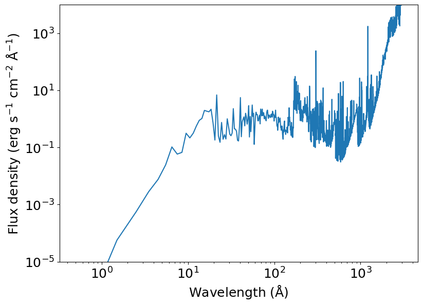
Next, we retrieve the high-energy spectrum of the host star with fluxes at the planet. For this example, we use the solar spectrum for convenience.
[3]:
units = {'wavelength': u.angstrom, 'flux': u.erg / u.s / u.cm ** 2 / u.angstrom}
spectrum = tools.make_spectrum_from_file('../../data/solar_spectrum_scaled_lambda.dat',
                                    units)
plt.loglog(spectrum['wavelength'], spectrum['flux_lambda'])
plt.ylim(1E-5, 1E4)
plt.xlabel(r'Wavelength (${\rm \AA}$)')
plt.ylabel(r'Flux density (erg s$^{-1}$ cm$^{-2}$ ${\rm \AA}^{-1}$)')
plt.show()
Now we can calculate the distribution of ionized/neutral hydrogen and the structure of the upper atmosphere.
[4]:
initial_f_ion = 0.0
r = np.logspace(0, np.log10(20), 100)  # Radial distance profile in unit of planetary radii

f_r, mu_bar = hydrogen.ion_fraction(r, R_pl, T_0, h_fraction,
                            m_dot, M_pl, mu_0, star_mass=M_star,
                            semimajor_axis=a_pl,
                            spectrum_at_planet=spectrum, exact_phi=True,
                            initial_f_ion=initial_f_ion, relax_solution=True,
                            return_mu=True)

vs = parker.sound_speed(T_0, mu_bar)  # Speed of sound (km/s, assumed to be constant)
rs = parker.radius_sonic_point_tidal(M_pl, vs, M_star, a_pl)  # Radius at the sonic point (jupiterRad)
rhos = parker.density_sonic_point(m_dot, rs, vs)  # Density at the sonic point (g/cm^3)

r_array = r * R_pl / rs
v_array, rho_array = parker.structure_tidal(r_array, vs, rs, M_pl, M_star, a_pl)
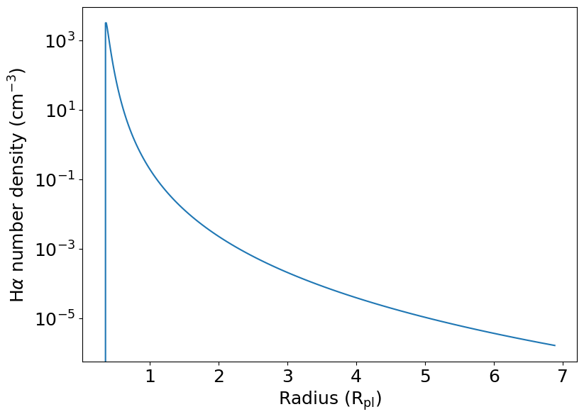
In the next step, we calculate the distribution of H atoms in the H\(\alpha\) transition (with an electron transitioning from state \(n=3\) to \(n=2\)). To this end, we need the electron density in unit cm\(^{-3}\), the neutral H number density in SI units, and the properties of the transition, which we get from the lines module.
[5]:
m_H = 1.008 * 1.67262192369e-24  # Hydrogen atomic mass in kg

# We assume that all electrons come from H ionization, so their number
# density is the same as the density of ionized H
n_e = (rho_array * rhos * h_fraction / (h_fraction + 4 * he_fraction) / m_H) * f_r * (1 / u.cm ** 3)

# Get the transition properties
lambda_alpha, n_alpha, f_alpha, g_alpha, a_alpha = lines.balmer_halpha_properties()

# Neutral H number density in SI units
n_H_0 = (rho_array * rhos * h_fraction / (h_fraction + 4 * he_fraction) / m_H)
n_H_0_SI = n_H_0 * 1E6
The radial distribution of H\(\alpha\) particles is given by the number density of neutral H multiplied by a scaling factor calculated using the Boltzmann and Saha equations. These are computer under the hood of the hydrogen.halpha_scale() function, as seen in the next cell.
[6]:
n_H_2n_scale = hydrogen.balmer_fraction(T_0, n_e, g_alpha, n_alpha)
n_H_2n = n_H_2n_scale * n_H_0_SI

plt.semilogy(r_array, n_H_2n)
plt.xlabel(r'Radius (R$_\mathrm{pl}$)')
plt.ylabel(r'H$\alpha$ number density (cm$^{-3}$)')
[6]:
Text(0, 0.5, 'H$\\alpha$ number density (cm$^{-3}$)')
Now that we have the 1-D profile of volumetric densities of the H\(\alpha\), we can calculate the spectroscopic transit signal using simplified ray tracing and radiative transfer. For now we will assume an impact factor of zero (so the planet is in the dead center of the star) and also a phase of zero (so the planet is at mid-transit phase). The phases of \(-0.5\) and \(+0.5\) correspond to the ingress and egress.
[7]:
# First convert everything to SI units because they make our lives
# much easier.
R_pl_physical = R_pl * 71492000  # Planet radius in m
r_SI = r * R_pl_physical  # Array of altitudes in m
v_SI = v_array * vs * 1000  # Velocity of the outflow in m / s
n_H_2n_SI = n_H_2n * 1E6  # Volumetric densities in 1 / m ** 3
planet_to_star_ratio = 0.12086

# Set up the ray tracing. We will use a coarse 100-px grid size,
# but we use supersampling to avoid hard pixel edges.
flux_map, t_depth, r_from_planet = transit.draw_transit(
    planet_to_star_ratio,
    planet_physical_radius=R_pl_physical,
    impact_parameter=impact_parameter,
    phase=0.0,
    supersampling=10,
    grid_size=100)
Now we can finally calculate the transmission spectrum using the transit.radiative_transfer_2d() function.
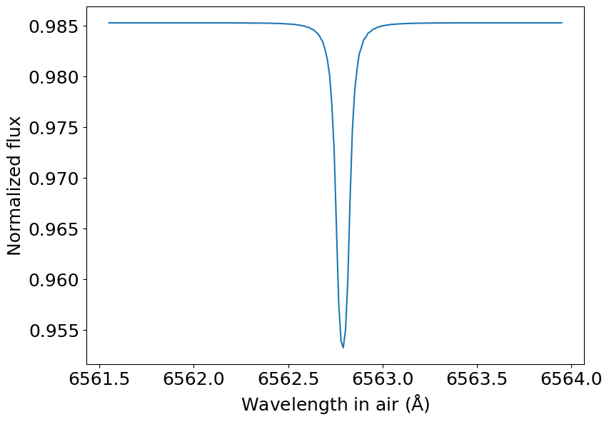
[8]:
wl = np.linspace(0.656155, 0.656395, 200) * 1E-6  # Wavelengths in m

spectrum = transit.radiative_transfer_2d(flux_map, r_from_planet, r_SI, n_H_2n_SI,
                                         v_SI, lambda_alpha, f_alpha, a_alpha,
                                         wl, T_0, m_H, wind_broadening_method='formal')

plt.plot(wl * 1E10, spectrum)
plt.xlabel(r'Wavelength in air (${\rm \AA}$)')
plt.ylabel('Normalized flux')
plt.show()