Exospheric metals
Some extremely hot planets may be in a state of hydrodynamic escape, in which the outflow of H is so intense, that it can drag up heavier species, like C and O to the upper atmosphere of the planet. In this notebook, we will use p-winds to quantify the amount of C and O in the exosphere of the hot Jupiter HD 209458 b using the modules carbon and oxygen (version 1.4.1 and onwards).
As always, let’s start by importing the necessary packages.
[1]:
import numpy as np
import matplotlib.pyplot as plt
import matplotlib.pylab as pylab
import astropy.units as u
import astropy.constants as c
from p_winds import tools, parker, hydrogen, helium, carbon, oxygen, lines, transit

pylab.rcParams['figure.figsize'] = 9.0,6.5
pylab.rcParams['font.size'] = 18
/home/docs/checkouts/readthedocs.org/user_builds/p-winds/envs/dev/lib/python3.11/site-packages/p_winds/tools.py:24: UserWarning: Environment variable PWINDS_REFSPEC_DIR is not set.
  warn("Environment variable PWINDS_REFSPEC_DIR is not set.")
We are going to replicate the quickstart example for HD 209458 b and include the tidal effects. We will assume that the planet has an isothermal upper atmosphere with temperature of \(9\,100\) K and a total mass loss rate of \(2 \times 10^{10}\) g s\(^{-1}\) based on the results from Salz et al. 2016. We will also assume: * The atmosphere is mostly
made up of H and He with number fractions \(0.9\) and \(0.1\), respectively * C and O are trace elements with solar abundance based on Asplund et al. 2009. p-winds uses these solar values by default, but they can be set by the user if preferred. * The H and He nuclei are fully neutral near the planet’s surface (this is going to be self-consistently calculated later). In the case of C, we assume they are fully
singly-ionized near the surface.
We will also need to know other parameters, namely: the stellar mass and radius, and the semi-major axis of the orbit.
[2]:
# HD 209458 b planetary parameters, measured
R_pl = 1.39  # Planetary radius in Jupiter radii
M_pl = 0.73  # Planetary mass in Jupiter masses
impact_parameter = 0.499  # Transit impact parameter
a_pl = 0.04634  # Orbital semi-major axis in astronomical units

# HD 209458 stellar parameters
R_star = 1.20  # Stellar radius in solar radii
M_star = 1.07  # Stellar mass in solar masses

# A few assumptions about the planet's atmosphere
m_dot = 10 ** 10.27  # Total atmospheric escape rate in g / s
T_0 = 9100  # Wind temperature in K
h_fraction = 0.90  # H number fraction
he_fraction = 1 - h_fraction  # He number fraction
he_h_fraction = he_fraction / h_fraction
mean_f_ion = 0.0  # Mean ionization fraction (will be self-consistently calculated later)
mu_0 = (1 + 4 * he_h_fraction) / (1 + he_h_fraction + mean_f_ion)
# mu_0 is the constant mean molecular weight (assumed for now, will be updated later)

# The trace abundances of C and O
c_abundance = 8.43  # Asplund et al. 2009
c_fraction = 10 ** (c_abundance - 12.00)
o_abundance = 8.69  # Asplund et al. 2009
o_fraction = 10 ** (o_abundance - 12.00)
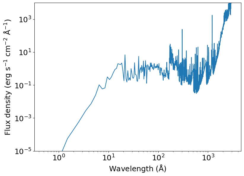
Next, we retrieve the high-energy spectrum of the host star with fluxes at the planet. For this example, we use the solar spectrum for convenience.
[3]:
units = {'wavelength': u.angstrom, 'flux': u.erg / u.s / u.cm ** 2 / u.angstrom}
spectrum = tools.make_spectrum_from_file('../../data/solar_spectrum_scaled_lambda.dat',
                                    units)
plt.loglog(spectrum['wavelength'], spectrum['flux_lambda'])
plt.ylim(1E-5, 1E4)
plt.xlabel(r'Wavelength (${\rm \AA}$)')
plt.ylabel(r'Flux density (erg s$^{-1}$ cm$^{-2}$ ${\rm \AA}^{-1}$)')
plt.show()
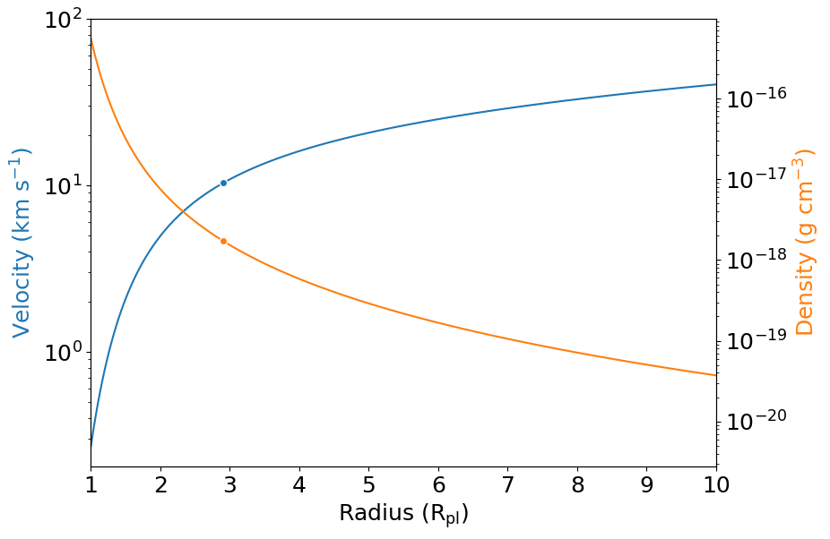
Now we can calculate the distribution of ionized/neutral hydrogen and the structure of the upper atmosphere.
[4]:
initial_f_ion = 0.0
r = np.logspace(0, np.log10(20), 100)  # Radial distance profile in unit of planetary radii

f_r, mu_bar = hydrogen.ion_fraction(r, R_pl, T_0, h_fraction,
                            m_dot, M_pl, mu_0, star_mass=M_star,
                            semimajor_axis=a_pl,
                            spectrum_at_planet=spectrum, exact_phi=True,
                            initial_f_ion=initial_f_ion, relax_solution=True,
                            return_mu=True)

f_ion = f_r
f_neutral = 1 - f_r

vs = parker.sound_speed(T_0, mu_bar)  # Speed of sound (km/s, assumed to be constant)
rs = parker.radius_sonic_point_tidal(M_pl, vs, M_star, a_pl)  # Radius at the sonic point (jupiterRad)
rhos = parker.density_sonic_point(m_dot, rs, vs)  # Density at the sonic point (g/cm^3)

r_array = r * R_pl / rs
v_array, rho_array = parker.structure_tidal(r_array, vs, rs, M_pl, M_star, a_pl)

# Convenience arrays for the plots
r_plot = r_array * rs / R_pl
v_plot = v_array * vs
rho_plot = rho_array * rhos

# Finally plot the structure of the upper atmosphere
# The circles mark the velocity and density at the sonic point
ax1 = plt.subplot()
ax2 = ax1.twinx()
ax1.semilogy(r_plot, v_plot, color='C0')
ax1.plot(rs / R_pl, vs, marker='o', markeredgecolor='w', color='C0')
ax2.semilogy(r_plot, rho_plot, color='C1')
ax2.plot(rs / R_pl, rhos, marker='o', markeredgecolor='w', color='C1')
ax1.set_xlabel(r'Radius (R$_{\rm pl}$)')
ax1.set_ylabel(r'Velocity (km s$^{-1}$)', color='C0')
ax2.set_ylabel(r'Density (g cm$^{-3}$)', color='C1')
ax1.set_xlim(1, 10)
plt.show()
We will also need the neutral and ion fractions of helium.
[5]:
# Calculate the helium ion fraction
f_he_plus = helium.ion_fraction(
    r, v_array, rho_array, f_ion,
    R_pl, T_0, h_fraction, vs, rs, rhos, spectrum,
    initial_f_he_ion=0.0, relax_solution=True)

# Hydrogen atom mass
m_h = c.m_p.to(u.g).value

# Number density of helium nuclei
he_fraction = 1 - h_fraction
n_he = (rho_array * rhos * he_fraction / (h_fraction + 4 * he_fraction) / m_h)
n_he_ion = f_he_plus * n_he
With all this setup done, we will proceed to calculate the number densities of neutral, singly-ionized and doubly-ionized C. We will assume that the C nuclei are all singly-ionized near the surface (so initial_f_c_ion is [1.0, 0.0]).
[6]:
f_c_ii, f_c_iii = carbon.ion_fraction(radius_profile=r,
                                      velocity=v_array,
                                      density=rho_array,
                                      hydrogen_ion_fraction=f_ion,
                                      helium_ion_fraction=f_he_plus,
                                      planet_radius=R_pl,
                                      temperature=T_0,
                                      h_fraction=h_fraction,
                                      c_fraction=c_fraction,
                                      speed_sonic_point=vs,
                                      radius_sonic_point=rs,
                                      density_sonic_point=rhos,
                                      spectrum_at_planet=spectrum,
                                      initial_f_c_ion=np.array([1.0, 0.0]),
                                      method='Radau',
                                      relax_solution=True)

# Number density of carbon nuclei
n_c = (rho_array * rhos * c_fraction / (h_fraction + 4 * he_fraction + 12 * c_fraction) / m_h)

n_c_i = (1 - f_c_ii - f_c_iii) * n_c
n_c_ii = f_c_ii * n_c
n_c_iii = f_c_iii * n_c

plt.semilogy(r, n_c_i, color='C0', label='C I')
plt.semilogy(r, n_c_ii, color='C1', label='C II')
plt.semilogy(r, n_c_iii, color='C2', label='C III')
plt.xlabel(r'Radius (R$_\mathrm{pl}$)')
plt.ylabel('Number density (cm$^{-3}$)')
plt.xlim(1, 10)
plt.ylim(1E-3, 1E7)
plt.legend()
plt.show()
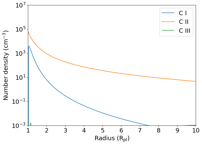
In the plot above we see that most of the C nuclei in the upper atmosphere of HD 209458 b are singly-ionized, with only a small fraction of them in neutral state by a factor of 3 orders of magnitude. Furthermore, doubly-ionized C are not present.
Next, we do the same exercise for oxygen. We will assume that all O nuclei are neutral near the surface at first.
[7]:
f_o_ii = oxygen.ion_fraction(radius_profile=r,
                             velocity=v_array,
                             density=rho_array,
                             hydrogen_ion_fraction=f_ion,
                             helium_ion_fraction=f_he_plus,
                             planet_radius=R_pl,
                             temperature=T_0,
                             h_fraction=h_fraction,
                             o_fraction=o_fraction,
                             speed_sonic_point=vs,
                             radius_sonic_point=rs,
                             density_sonic_point=rhos,
                             spectrum_at_planet=spectrum,
                             initial_f_o_ion=0.0,
                             relax_solution=True)

# Number density of oxygen nuclei
n_o = (rho_array * rhos * o_fraction / (h_fraction + 4 * he_fraction + 16 * o_fraction) / m_h)

n_o_i = (1 - f_o_ii) * n_o
n_o_ii = f_o_ii * n_o

plt.semilogy(r, n_o_i, color='C0', label='O I')
plt.semilogy(r, n_o_ii, color='C1', label='O II')
plt.xlabel(r'Radius (R$_\mathrm{pl}$)')
plt.ylabel('Number density (cm$^{-3}$)')
plt.xlim(1, 10)
plt.ylim(1E-3, 1E7)
plt.legend()
plt.show()
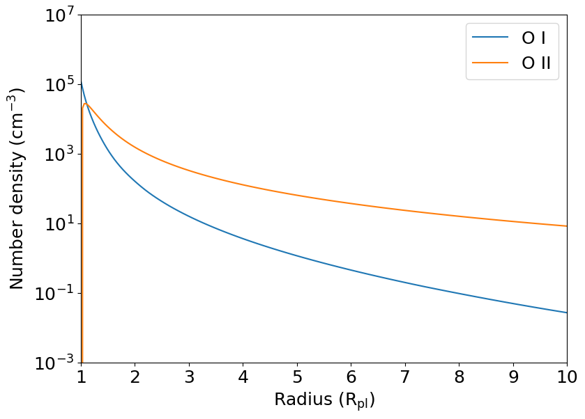
And there we see that most of the oxygen nuclei are singly-ionized, except in the innermost upper atmosphere layers, where neutral oxygen dominates.
For the next part of this tutorial, we will estimate the in-transit absorption profiles for the relevant wavelengths in real observations. These exospheric carbon and oxygen lines are located in the ultraviolet, which are accessible only with the Hubble Space Telescope.
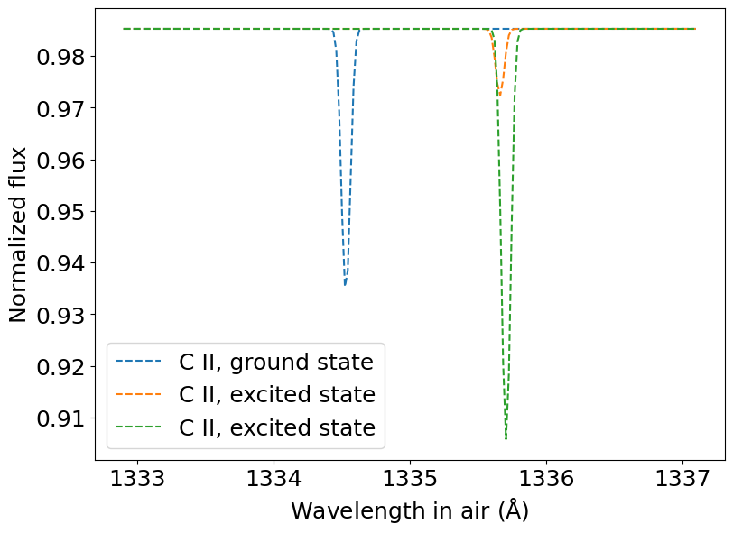
The tricky part of the C II triplet is that the line at 133.4 nm arises from the ground state, and the other two at 133.5 nm are a doublet arising from the first excited state. The number density of C II we calculated above assumes that all nuclei are in the ground state, and we need to estimate how many of them are in the excited state as well.
There are a few ways of calculating the population of C II nuclei. I used the `ChiantiPy code <https://github.com/chianti-atomic/ChiantiPy/>`__, and estimated that, for the exosphere of HD 209458 b (temperature 9100 K and density of electrons \(\sim 6 \times 10^6\) cm\(^{-3}\)), we have roughly 33% of C II ions in the ground state, and 66% in the excited state.
[8]:
# Set up the ray tracing. We will use a coarse 100-px grid size,
# but we use supersampling to avoid hard pixel edges.
# We convert everything to SI units because they make our lives
# much easier.
R_pl_physical = R_pl * 71492000  # Planet radius in m
r_SI = r * R_pl_physical  # Array of altitudes in m
v_SI = v_array * vs * 1000  # Velocity of the outflow in m / s
n_c_ii_SI = n_c_ii * 1E6  # Volumetric densities in 1 / m ** 3
planet_to_star_ratio = 0.12086

flux_map, t_depth, r_from_planet = transit.draw_transit(
    planet_to_star_ratio,
    planet_physical_radius=R_pl_physical,
    impact_parameter=impact_parameter,
    phase=0.0,
    supersampling=10,
    grid_size=100)

# Retrieve the properties of the C II lines; they were hard-coded
# using the tabulated values of the NIST database
# wX = central wavelength, fX = oscillator strength, a_ij = Einstein coefficient
w0, w1, w2, f0, f1, f2, a_ij_0, a_ij_1, a_ij_2 = lines.c_ii_properties()

m_C = 12 * 1.67262192369e-27  # Carbon atomic mass in kg
wl = np.linspace(1332.9, 1337.1, 200) * 1E-10  # Wavelengths in Angstrom

method = 'average'

spectrum_0 = transit.radiative_transfer_2d(flux_map, r_from_planet,  # Ground state
                                        r_SI, n_c_ii_SI * 0.33, v_SI, w0, f0, a_ij_0,
                                        wl, T_0, m_C, wind_broadening_method=method)
spectrum_1 = transit.radiative_transfer_2d(flux_map, r_from_planet,  # Excited state
                                        r_SI, n_c_ii_SI * 0.66, v_SI, w1, f1, a_ij_1,
                                        wl, T_0, m_C, wind_broadening_method=method)
spectrum_2 = transit.radiative_transfer_2d(flux_map, r_from_planet,  # Excited state
                                        r_SI, n_c_ii_SI * 0.66, v_SI, w2, f2, a_ij_2,
                                        wl, T_0, m_C, wind_broadening_method=method)

plt.plot(wl * 1E10, spectrum_0, ls='--', label='C II, ground state')
plt.plot(wl * 1E10, spectrum_1, ls='--', label='C II, excited state')
plt.plot(wl * 1E10, spectrum_2, ls='--', label='C II, excited state')
plt.legend()
plt.xlabel(r'Wavelength in air (${\rm \AA}$)')
plt.ylabel('Normalized flux')
plt.show()
And now for the oxygen lines. Similarly, the first line is a resonant line, and the other two are doubles arising from two different excited states.
From ChiantiPy, the ratios for the ground state, the first and second excited states are 0.85, 0.10 and 0.05.
[9]:
n_o_i_SI = n_o_i * 1E6  # Volumetric densities in 1 / m ** 3

# Retrieve the properties of the O I triplet; they were hard-coded
# using the tabulated values of the NIST database
# wX = central wavelength, fX = oscillator strength, a_ij = Einstein coefficient
w0, w1, w2, f0, f1, f2, a_ij_0, a_ij_1, a_ij_2 = lines.o_i_properties()

m_O = 16 * 1.67262192369e-27  # Oxygen atomic mass in kg
wl = np.linspace(1300.9, 1307.1, 200) * 1E-10  # Wavelengths in Angstrom

method = 'average'

spectrum_0 = transit.radiative_transfer_2d(flux_map, r_from_planet,  # Ground state
                                        r_SI, n_o_i_SI * 0.85, v_SI, w0, f0, a_ij_0,
                                        wl, T_0, m_O, wind_broadening_method=method)
spectrum_1 = transit.radiative_transfer_2d(flux_map, r_from_planet,  # First excited state
                                        r_SI, n_o_i_SI * 0.10, v_SI, w1, f1, a_ij_1,
                                        wl, T_0, m_O, wind_broadening_method=method)
spectrum_2 = transit.radiative_transfer_2d(flux_map, r_from_planet,  # Second excited state
                                        r_SI, n_o_i_SI * 0.05, v_SI, w2, f2, a_ij_2,
                                        wl, T_0, m_O, wind_broadening_method=method)

plt.plot(wl * 1E10, spectrum_0, ls='--', label='O I, ground state')
plt.plot(wl * 1E10, spectrum_1, ls='--', label='O I, first excited state')
plt.plot(wl * 1E10, spectrum_2, ls='--', label='O I, second excited state')
plt.legend()
plt.xlabel(r'Wavelength in air (${\rm \AA}$)')
plt.ylabel('Normalized flux')
plt.show()
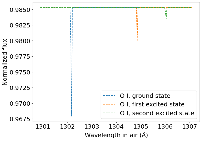
What we can conclude from this exercise is that, if we assume a Parker-wind like escape for HD 209458 b, solar abundances of C and O, and a solar-like high-energy spectrum for the host star, then the excess in-transit signature of neutral O will be about 0.5% in the core of the strongest O I line in the UV. For C II, a much promising signature stronger than 7.5% will be present in the strongest line of the transmission spectrum.